Databases are the main way that large organizations store data that needs to be analyzed. But databases don’t just store the data, they also allow you to work with it: ask questions by running queries, create new combinations of facts by joining tables, all to understand what is in the data and to better inform business decisions.
In this post we cover some basics of databases including core terminology, an introduction to tables (and how data is structured in them), and the basics of keys and joins. We’ll draw some comparisons to spreadsheets, since that is the other common format in which people encounter data.
This initial post will set you up to dive into our upcoming blog posts on basic data analysis in databases using queries and joins.
What are relational databases?
Most databases you will encounter in business contexts are called relational databases, hence also the slightly old-school acronym RDMS for relational database management system (also sometimes called RDBMS, using the two letters DB for database). But what exactly does it mean for a database to be relational?
In a relational database, data is stored in tables. This is much like in Excel, however the format between the tables is quite different. Each row in a database table is treated as an independent piece of data, and is in itself a relation: it combines a set of attributes (in the columns) that taken together describe one thing or data item (like a sale).
The table of pizza orders shown below is from our Pizza Paradise dataset. The IDs in the first three columns might look cryptic at first, but I picked this example on purpose. It’s a better representation of the kinds of data tables you’ll likely encounter than a nicer-looking example.
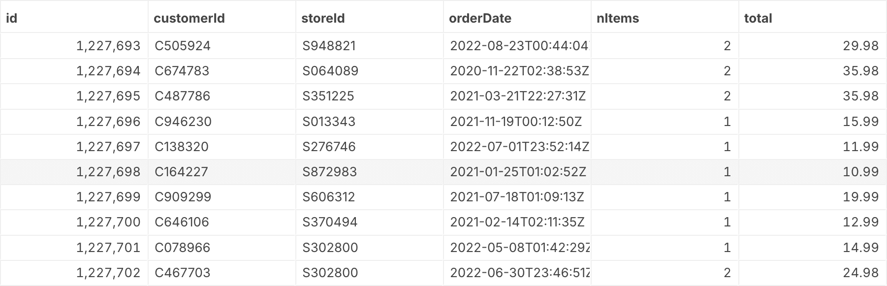
This table contains orders, and for each it has an identifier for the order (which is also the key for this table, we’ll get to that below), IDs for the customer and store involved in the order, an order date, a number of items, and a total amount.
Each row here is a relation, tying together the various attributes (like customer IDs, order date, etc.) with the order ID. Rows are identified not by their position in the table, but by a key. In this case, the key is simply the order ID in the first column, but it can be more complex. We'll talk a little bit more about keys below.
In Excel, you’re probably used to defining operations between rows, where you can rely on the ordering being stable. In databases, by contrast, the ordering of rows is completely arbitrary, and not fixed. In the example above, it appears to be based on order ID, but we could just as well order by date or total amount. This more flexible data model also allows for much easier aggregation operations to get totals by store, or by month, but we’ll get to those in a future post.
Table shapes and normal forms
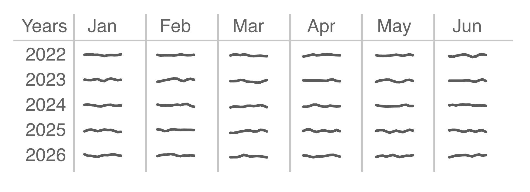
Databases also differ from spreadsheets in their shape. Spreadsheets are usually organized in a two-dimensional way, where one dimension (like the month) goes across the columns, and another (like the year) across the rows.
This kind of organization makes sense in a spreadsheet, where it’s often interesting to compute values (like sums or averages) across both rows and columns: sum of sales across a year, average sales over the months of a year.
Database tables, by contrast, are usually organized in a way that favors more rows over more columns. This is sometimes called the “long and skinny” format (as opposed to the “short and wide” of spreadsheets), or more formally a normal form. In statistics, this is also known as tidy data.
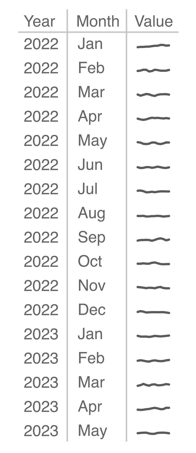
Instead of a column for each month and a row for each year, a database table has columns for the year and month, and then rows for each combination of the two. The same would be true if we were looking at products: instead of a column for each product, there would be a single column called ‘product’ containing the names of the products, requiring many more rows.
This data structure is the core of the relational model. We end up with a lot more rows, but this way allows us to organize data not just in two dimensions, but over a much larger number of dimensions and for as many attributes as we want.
The difference between fact tables and dimension tables
Let’s look at the pizza orders example from the top of this post again. I mentioned that it looks kind of cryptic with all these IDs. Who exactly is customer C505924? And where would you find store S948821?
While this might seem odd at first, it is the consequence of a core organizational principle of databases in normal form: data is split into fact tables and dimension tables.
The example above is a fact table, which connects a number of different types of information (customers, stores, and order data). The details of each customer and store live in dimension tables, which are linked through their respective IDs. The advantage of separating data into fact and dimension tables is that we have to keep each customer and store’s information only once in the dimension tables, rather than hundreds or thousands of times as attributes in the fact table. That system also gives us more consistency, because we won’t suddenly find the same store with different addresses or ZIP codes.
Understanding database keys and joins
The way fact and dimension tables are connected is through keys. We’re not going to cover the joining of tables in this post, but it’s important to have an idea of the basic concept to understand why databases are organized like this.
A key is generally a unique attribute (or set of attributes) that allows a database to find a particular row in a table. The easiest way to do this is to assign each row a unique identifier, like the order ID in the first column in the pizza orders example above. The key can also be a combination of multiple values.
A join then allows us to create a new table by looking up the IDs that are found in a fact table, and inserting the information from the dimension table instead. So again using the pizza orders, the database would look up which store has ID = S948821 and insert its address, and look up which customer has ID = C505924 and insert the name. That might then give us the information to print out a receipt. Or we could look up the customer’s age group and the store’s ZIP code, and count how many times each combination occurs. That might tell us something about the different customer demographics in different areas.
If this all seems confusing, don’t worry. We’ll get into joins in much more detail in the coming posts.
Databases are your friends!
Databases might seem difficult and unfamiliar at first, but like spreadsheets and simple data files, they just require some understanding of core concepts I covered here like “long and skinny” data, keys, and types of tables. Most data lives in databases, certainly when it comes to larger amounts of data, so knowing your way around them is always going to be a plus for data analysis.
Come back soon! We’ll get into more detail about how table joins and data transformation in databases work in upcoming posts.