Databases allow you to both store your data and answer a variety of questions about your data. In a previous post, we covered how database tables are structured and why databases look different from spreadsheets. In this post, we’ll take a closer look at the kinds of questions you can ask of a single table, and start to analyze our data. We’ll start with simple questions like counting the number of rows, and then move on to more aggregations like sums and averages, and how to compute those for different groups in the data. At the end, we’ll also cover filtering data to select rows by a criterion.
SQL, the Structured Query Language (usually pronounced “sequel”), is the main way to talk to relational databases. Being able to write some basic SQL queries, or at least read and understand them, is a useful skill for anyone working with data. It also seems a bit silly to talk about database queries and not show the code, which is why we’re including it here.
The goal of this post is not to teach you the intricacies of SQL. SQL can get pretty involved, so in this post we only cover simple queries that are quite straightforward. If you don’t care about SQL, you can skip them and still learn about the basic ideas.
Let’s count!
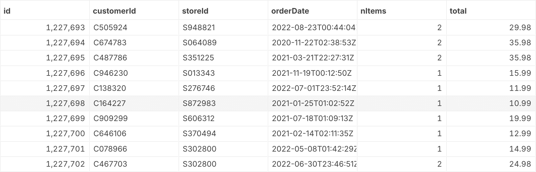
To start, we’ll build the simplest query to count our records in our database. We’ll be using the same table of orders at a fictional pizza chain as last time, which looks like this:
How many orders do we have in our dataset? To find out, we’ll write a SQL query that performs a count operation.
Simple SQL queries generally look like “SELECT <stuff> FROM <table>”, and we’re using the COUNT() function here to perform the count. Since SQL is an old-school language from the 1980s, it’s common to capitalize all SQL keywords, which I’ll do here for clarity. You don’t have to do that if you feel like that’s too shouty, though.
We can also give the result of the COUNT() function a name so we can use it for other purposes later, that’s what the “AS numOrders” part is for. What are we selecting from? The pizzaOrders table! Since this is the result of a database query, it is shown as a table, even if we’re only getting a single value back.
SELECT COUNT(*) AS numOrders
  FROM pizzaOrders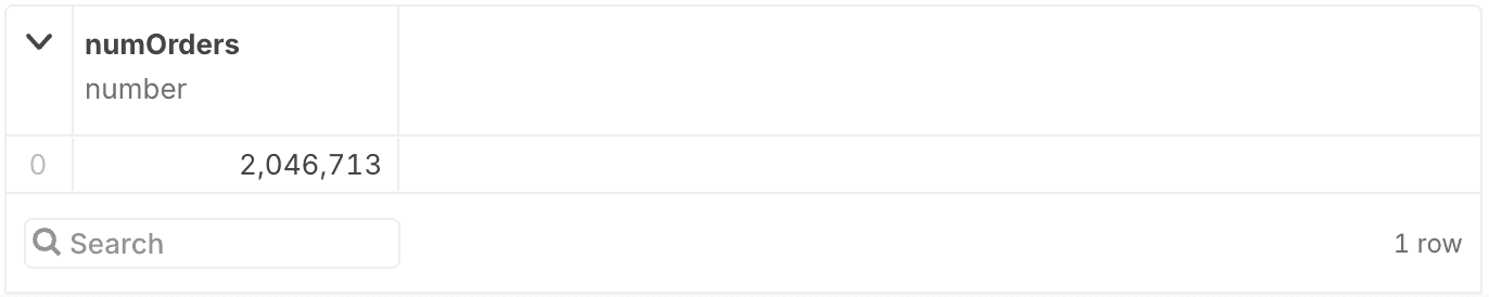
So now we know that we have about two million records in total, across all our locations. How many stores do we even have? You may be wondering about the asterisk in “COUNT(*),” which basically means “count everything.” Instead, we can count specific things, like the number of unique store IDs. SQL calls this DISTINCT, so instead of COUNT(*), we can use COUNT(DISTINCT storeId) to get the number of stores.
SELECT COUNT(DISTINCT storeId) AS numStores
  FROM orders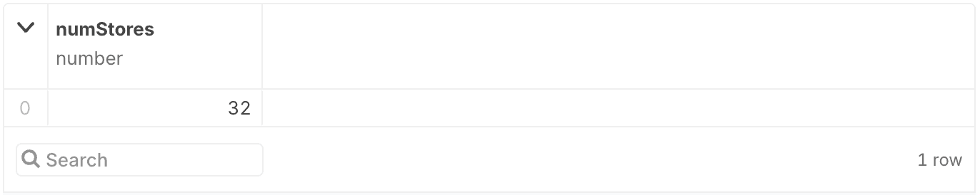
We can do the exact same thing with the customer ID to find out how many customers we’ve had:
SELECT COUNT(DISTINCT customerId) AS numCustomers
  FROM orders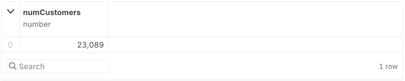
Now that’s great, I hear you say, but what if I want to know how many sales were made by each store? To find out, we can group the results by the store ID, so we don’t just get a single count, but instead the count for total sales for each store.
We’ll go back to using COUNT(*) here to count all the sales, but now we’ll include the storeId in the query, then use a GROUP BY clause to create separate counts for each store.
SELECT storeId, COUNT(*) AS numOrders
  FROM orders
  GROUP BY storeId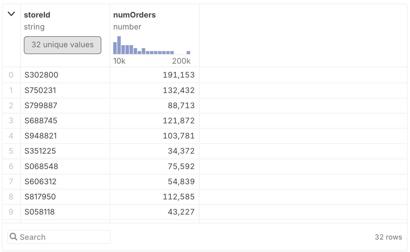
So now instead of a single value as the response, we get a table. It shows the store IDs in one column, and the order counts in the other. We call this aggregation because we’ve reduced the total ~2 million records for each order to just 32, one for each store.
The table here is just showing the first ten results, and you might have noticed that there doesn’t seem to be an obvious ordering. It’s not by ID, and it’s not by count. This goes back to what I said in the previous post about the order of rows or relations in a table not being fixed. When you perform a query, there’s no way to know what order the results will come out in.
We can, however, specify how we want the results to be sorted using an ORDER BY clause. This works the same as GROUP BY, in that we can specify any of the columns in the query as the sort criterion – including ones we’ve created in the query, like numOrders. However, by default, ORDER BY sorts in ascending order, from the smallest to the largest numbers. You often want descending order to see the largest numbers or highest counts, which is done by adding DESC just after the column name you’re sorting on.
SELECT storeId, COUNT(*) AS numOrders
  FROM orders
  GROUP BY storeId
  ORDER BY numOrders DESC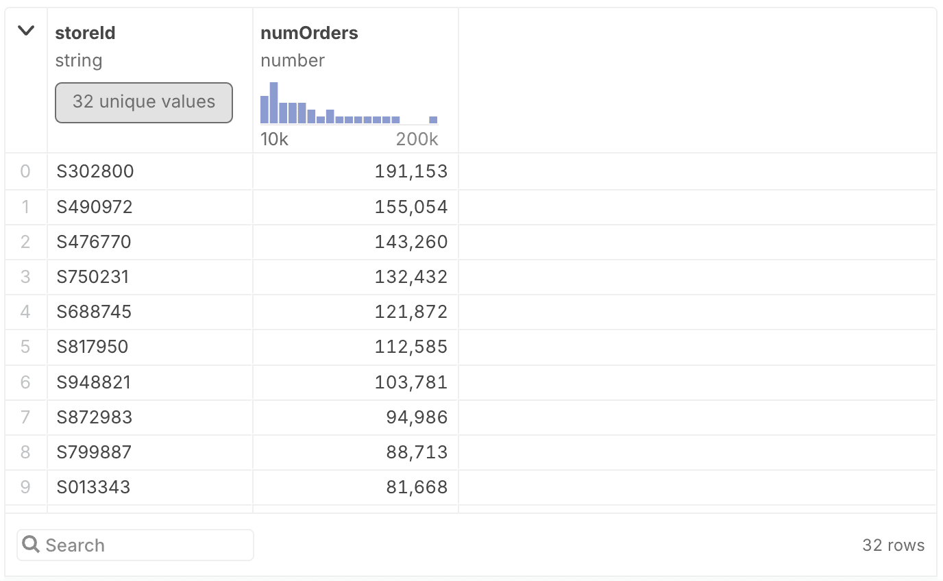
Computing totals and averages
If that was your first experience with SQL, just counting was a lot! But the good news is that computing other values is very similar, so we can use the same patterns to do that.
First, let’s see what the total revenue of all our sales was for the time period covered in this table. Instead of COUNT(), we’ll use SUM() to add up order prices from the total column, and everything else stays the same.
SELECT SUM(total) AS ordersTotal FROM orders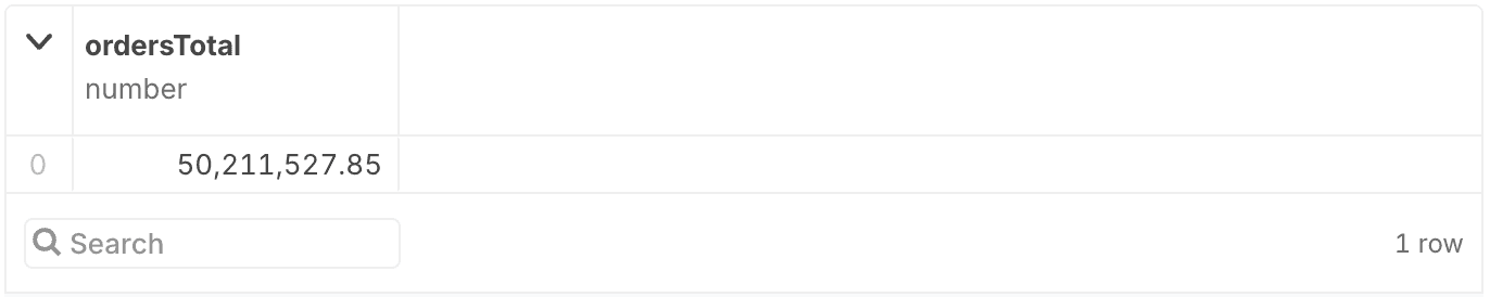
As before, we can break this down by store and sort in descending order, using GROUP BY and ORDER BY.
SELECT SUM(total) AS ordersTotal FROM orders
  GROUP BY storeId
  ORDER BY ordersTotal DESC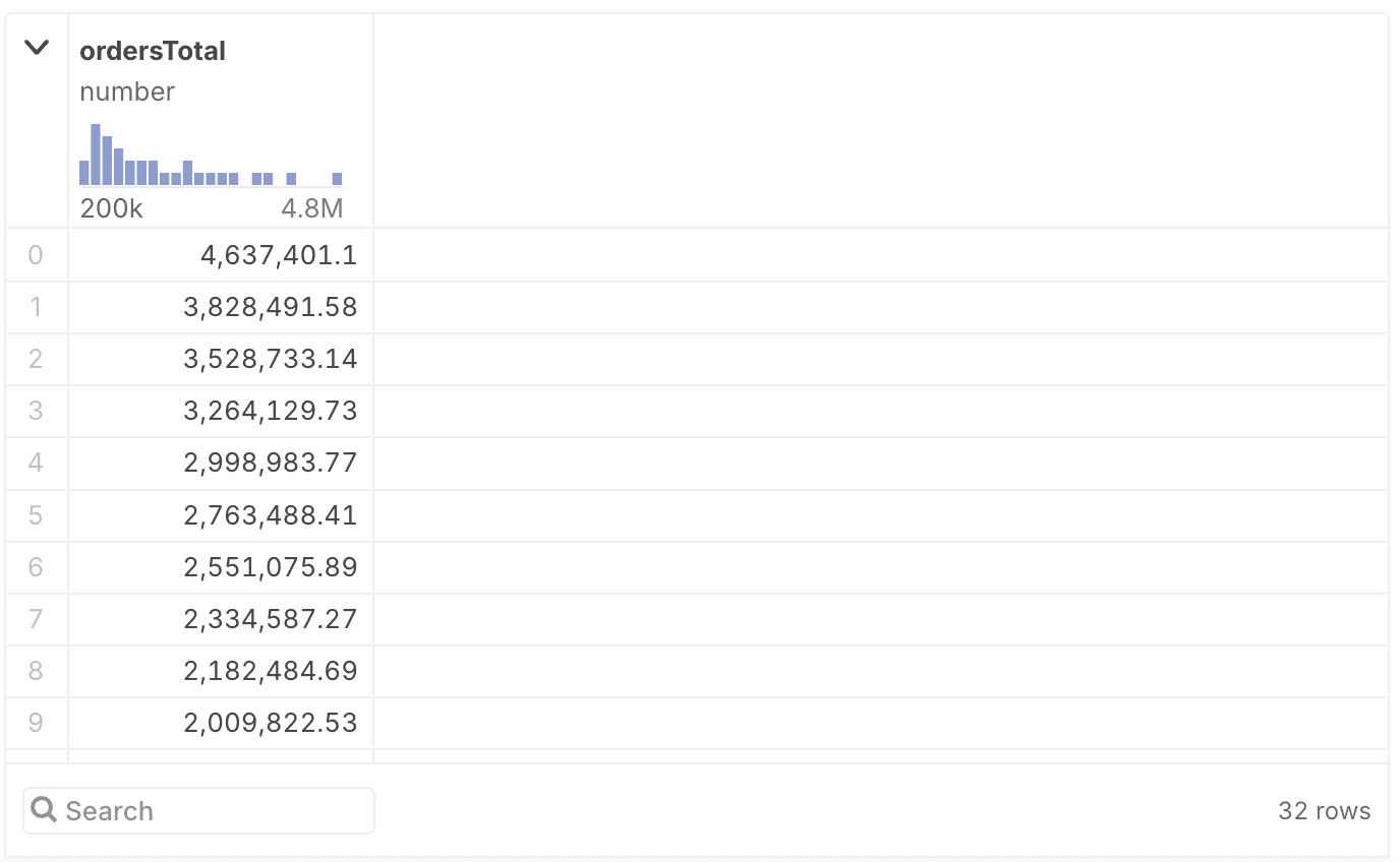
If you compare this to the final example in the section above, the only differences are that we’re using SUM instead of COUNT, and the name of the sum is different. Everything else is the same, since the structure of the query is the same: break down the table by store ID, then compute the sum (in this case, or the count above) for each, and then sort the results by the computed value.
There are many functions other than SUM to perform common operations, such as AVG for the average, and MIN and MAX. For example, we found the total sales for each store above. But what time period does our dataset even cover? We can find out with this simple query that selects the minimum and maximum order dates, and calls them first and last, respectively.
SELECT min(orderDate) AS first, max(orderDate) AS last FROM orders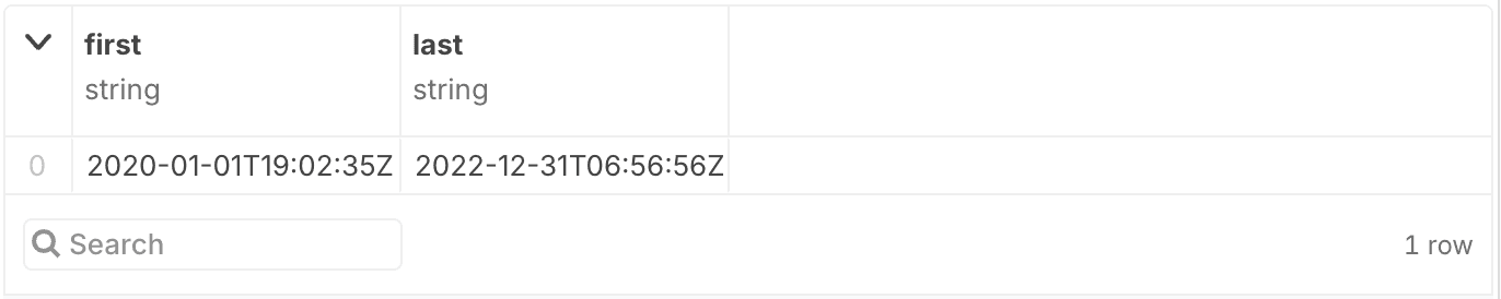
This kind of simple minimum and maximum query is also useful to look for outliers or special values. There are also functions to aggregate dates so we could compute sales by month or year in addition to (or instead of) the stores.
Filtering data
In addition to aggregating data, another operation databases do really well is filtering, which is done in SQL by adding a WHERE clause containing your condition. For example, the query below returns only orders over $100.
SELECT *
  FROM orders
  WHERE total > 100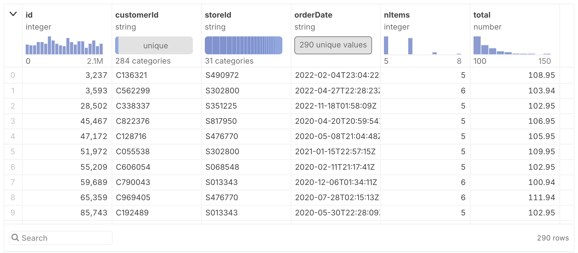
Again, we’re getting an unsorted list of orders by default, and perhaps we don’t even want to see each individual order – we may just want to find out how many orders exceeded $100. In that case, we’d want to count them by adding a COUNT clause.
SELECT COUNT(*) AS numOrders
  FROM orders
  WHERE total > 100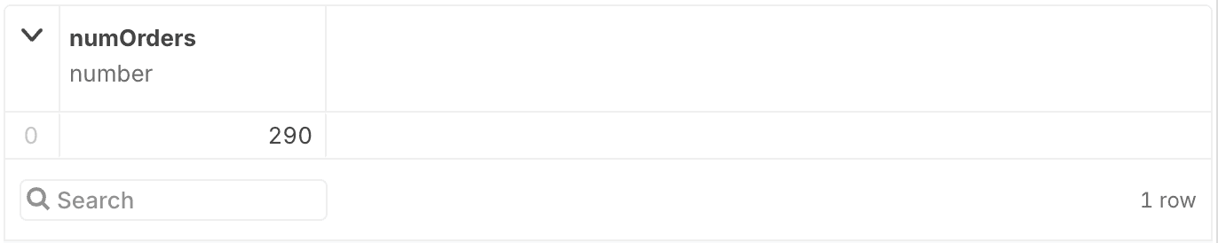
This clause can also be combined with the other pieces we’ve already used, for example to count how many orders over $100 were recorded by each store, and then sort the stores by that count. We use the same aggregation (GROUP BY) and sort (ORDER BY) clauses, and just add a WHERE clause. The WHERE applies before the aggregations, so this filters the data to only those rows with a total of over 100, and then does the counting from there.
SELECT storeId, COUNT(*) AS numOrders
  FROM orders
  WHERE total > 100
  GROUP BY storeId
  ORDER BY numOrders DESC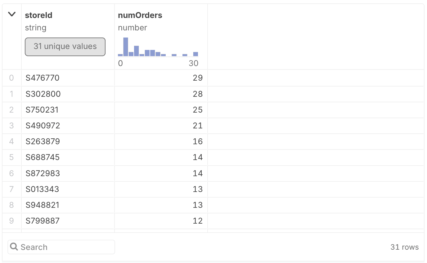
Filtering is incredibly important when doing data analysis to exclude special (or erroneous) values, and to restrict the query to a known time range or subset.
Unleash the power of databases!
There is a lot more that can be done here of course, but this should give you a sense of what is possible when analyzing databases. Queries can be combined to ask a variety of different questions, and we’ve only even used a single table so far. AI is making it even easier to build and edit more complex queries with text-to-SQL. Learn how to responsibly use AI for fast exploratory data analysis, while avoiding common pitfalls: