Histograms are essential for data exploration. So much so, that most graphical and statistical software allow users to create them with a single click or command. Both common and useful in business intelligence, histograms are often the first data visualization an analyst creates when exploring metrics like customer lifetime value, acquisition cost, and session lengths of website visits.
Histograms visualize the frequency distributions of numeric variables, with bars representing the binned counts of observations over a range of values. They provide a clear and intuitive look into the shape of the data, giving viewers a quick look at important characteristics like skew, modality (e.g. unimodal or bimodal), and outliers.
Designing default histograms may sound like a straightforward task. After all, all it takes is determining a reasonable number of bins, counting up the observations in each, and plotting the counts as vertical bars…right?
Wrong.
Behind the scenes, a number of careful decisions go into building useful histograms that work well for a wide range of data — and there’s a surprising amount of gray area to navigate along the way. Here we describe three interesting challenges we encountered, and how we decided to handle them, while designing out-of-the-box histograms in Observable Canvases.
Handling outliers
In business analytics, finding a normal and mesokurtic distribution is rare. You’re more likely to encounter skewed distributions, with most values bunched together on one end and a small number of values extending out in distant tails.
For example, the histogram below shows the distribution of product prices for a random sample of 200,000 Amazon e-commerce purchases:
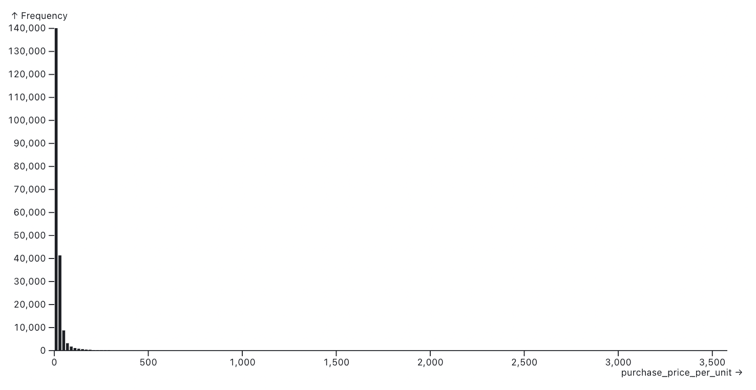
Outliers can expand the x-axis scale far beyond a range where the bulk of observations exist, resulting in largely empty histograms with just a few visible bars. Data: Berke et al. 2024.
This histogram isn’t wrong. But it also isn’t particularly useful — or nice to look at.
The issue is that the full range of product prices shown on the x-axis (maximum: $3,579) extends far beyond the range within which most observations exist, which looks to be between about $0 and $200. As a result, the majority of values are cramped into a handful of narrow bars, while the rest of the chart area looks like wasted blank space.
Given this common scenario, we wanted to design histograms that give viewers a more informative look at most of the data, while (1) delivering an honest representation of the overall distribution, and (2) without crudely chopping off the tails.
We landed on the following approach in Observable Canvases, which gives more space to the bulk of the data while still providing useful information about the range and number of outliers that lie beyond:
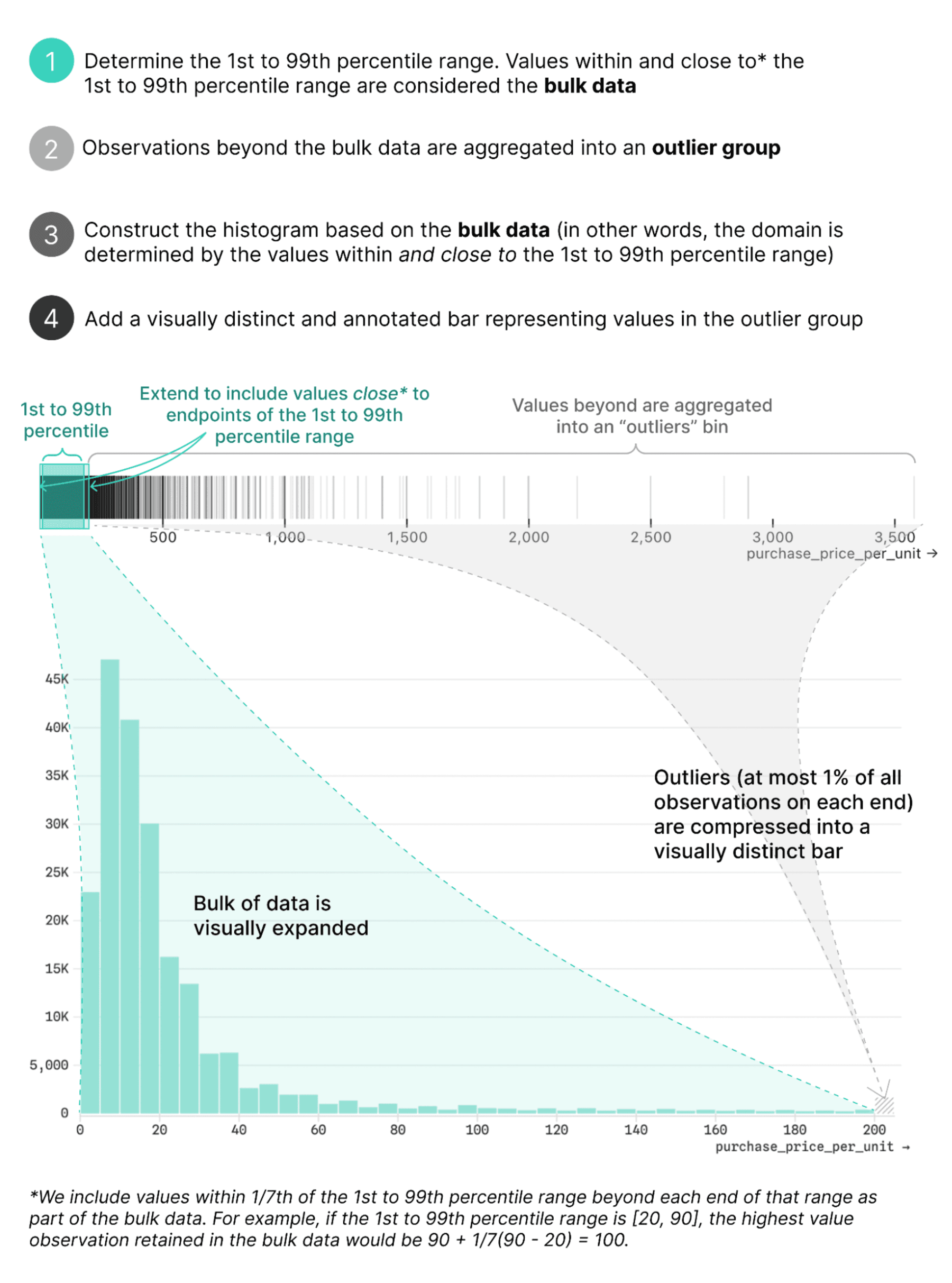
Since values between the 1st and 99th percentile are always included as part of the bulk data determining the histogram domain, at most 1% of observations on each end — and often less than that — are contained within the outlier bars. We include values beyond the 1st and 99th percentiles so that observations at or close to the bounds of that range are not excluded based solely on position. For example, if the first 1,000 values are all zeroes, and the 1st percentile occurs at zero #372, it wouldn’t make sense to segregate the first 371 zeroes as outliers in a separate bin.
The outlier bin differs from the others in an important way: its width, though equal in pixels to the others in the histogram, actually encompasses the entire range of outlier values. That’s why it’s crucial to make the outlier bin visually distinct (which we do using gray, hatched styling), and to provide more information about the values it contains.
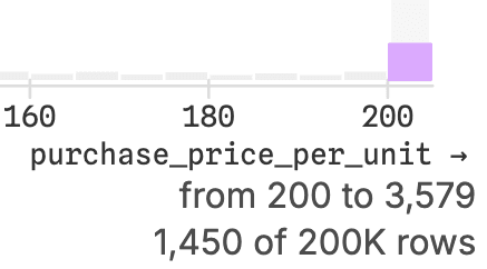
In a canvas, brushing over the outlier bin in the histogram above reveals both the count (n = 1,450, or 0.725% of all values) and total range of values ($200 to $3,579) it contains:
Are there tradeoffs? Sure! Do we think this is the one “correct” way? No!
Any time we rescale different pieces of the data in different ways, it creates room for misinterpretation. And, there are times when a viewer will want to see an expanded view of outliers. However, we think this approach strikes a nice balance between a clearer and more informative look into most of the data, while still keeping outliers in sight.
Making sure small counts don’t disappear
The strategy above addresses an x-axis issue, but there’s also a common y-axis issue in histogram design: the disappearance of small counts. When a bar representing a small count is plotted alongside much larger bars on a linear scale, it can become indistinguishable from a completely empty bin.
For example, the histogram below shows the distribution of commercial electricity rates across different U.S. zip codes. Due to the relatively large y-axis scale, the bar of height 7 (red arrow) is indistinguishable from the bar of height 0 to its right (blue arrow).
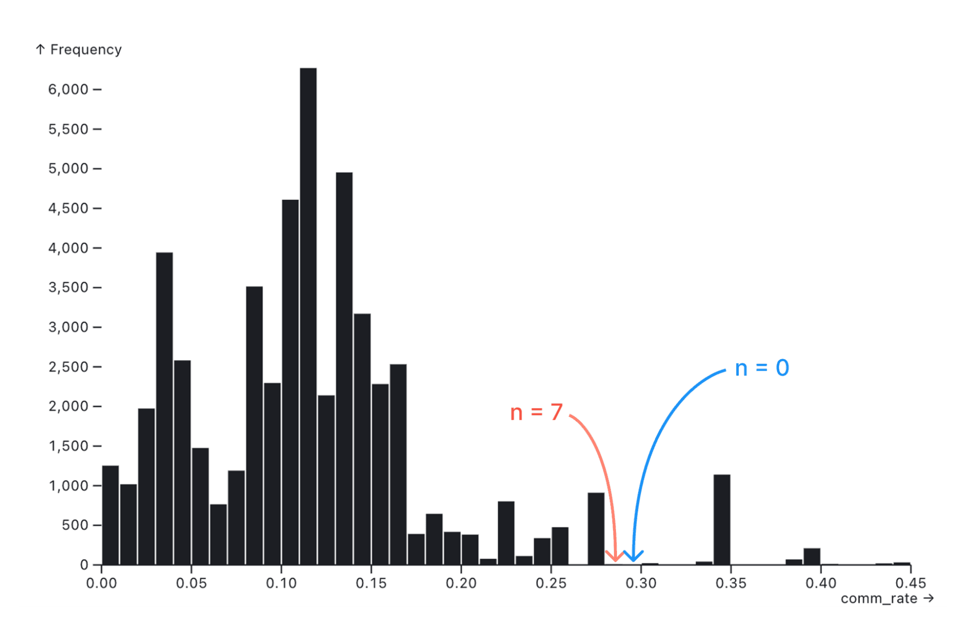
In exploratory data analysis, it’s hard to know what data to dig into further if you don’t even know where data exists. That’s why we think it’s important for viewers to see the difference between nothing and something — even if that something is very small.
We explored a number of approaches to uncovering these small but extant bins.
One option we considered was log transforming counts to compress the y-axis scale and give more ink to smaller bins. But log transforms and scales are notoriously hard to interpret, and can leave viewers with a false sense of parity between counts that are actually quite different. And, as a kicker, there’s that nagging math issue that arises when you have bins with n = 0 (since log(0) is undefined), which inspires some creative workarounds.
Ultimately, we decided to stick with untransformed counts and a linear y-axis scale. But, we still thought it necessary to visually distinguish between bars with n = 0, and n > 0.
We landed on setting an absolute minimum pixel height for any bars with a non-zero count. The histogram below highlights the same bins as shown above. But now, we can see a small bar is visible in the n = 7 bin:
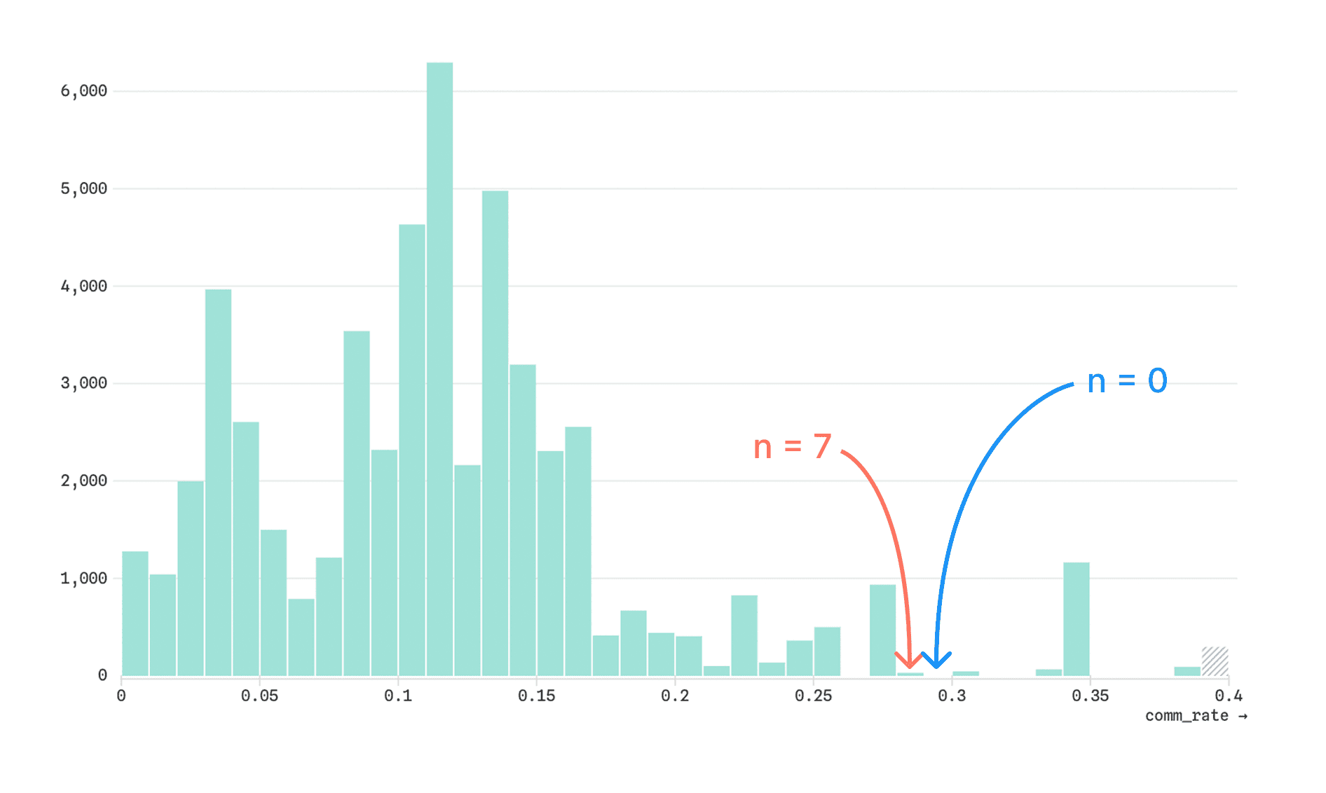
This approach to differentiating between empty bins and those with very low counts gives viewers a visual indication of where data exists, without drastically changing the look or interpretation of the overall distribution.
Choosing between continuous and discrete histograms
Histograms are often used to visualize the distribution of continuous quantitative variables like temperature, electricity usage, or file size. But, quantitative data can also be discrete, meaning that observations only exist at certain values. Often these are counts. For example, a political survey might ask participants how many children they have. The resulting data is discrete because values are limited to non-negative integers (0, 1, 2, etc.).
With discrete quantitative values, it often makes more sense to show a bar for each unique value, rather than aggregating multiple values into broader bins like we do in continuous histograms. That’s especially true if there only exist a relatively small number of unique values. For example, the histogram below shows the distribution of household size (number of people) based on 41,569 survey responses in San Francisco:
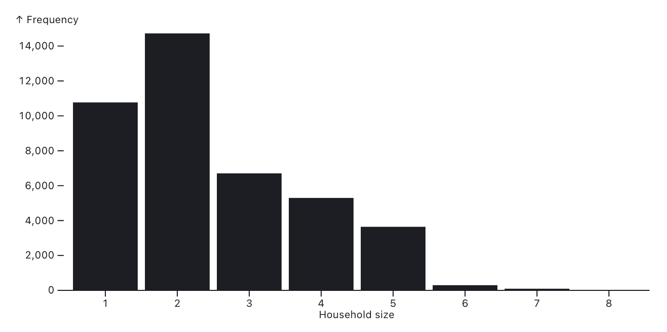
Discrete histograms visualize the frequency of each unique value in a separate bar, rather than binning counts across a continuous range, as shown here for household size in San Francisco. Data: San Francisco City Survey Data.
When we ask a BI visualization tool to create a histogram, however, it only sees a series of numbers. It has no sense of the methodology, or domain expertise, needed to determine whether the underlying variable is discrete or continuous. So a visualization tool can’t know for certain whether a histogram should be continuous or discrete.
We can, however, make an educated guess about which is a better default option based on characteristics of the data.
In canvases, we include some simple logic to determine whether we generate a continuous or discrete histogram. Our conditions for defaulting to discrete are as follows:
Fewer than 20 bins total
For each non-outlier bin, the minimum value is equal to the maximum value, ensuring that each bin represents a single value
Bins are not fractional
With those rules in place, we can see the two different types of charts created in a canvas, depending on the selected data.
Building a histogram with Observable Plot
Want to try building a histogram? With Observable Plot, it only takes a few lines ofJavascript code to get started. Jump into an Observable Notebook, drop in your data, and search for “histogram” in the new cell menu, or copy and paste the code snippet below into a JavaScript cell. Once you’ve replaced the dataset_name and variable_name with your own, you’re on your way to a custom histogram!
Plot.plot({
  marks: [
    Plot.rectY(dataset_name, Plot.binX({ y: "count" }, { x: "variable_name" })),
    Plot.ruleY([0])
  ]
})
Explore more built-in charts in Observable Canvases
Histograms are extremely useful and common charts to explore data distributions for business analytics. In canvases, we’ve designed generalizable histograms that can give you a better first look at the bulk of your data, ensure that small bins aren’t hidden from view, and default to a discrete or continuous chart based on characteristics of the data.
Learn how you can do fast, visual analytics in our new collaborative canvases, and sign up for early access to canvases today.