Creating a data visualization seems simple enough, until you realize how a decision like selecting a chart can impact your ability to communicate insights effectively. Selecting the right type of chart, and making smart design decisions along the way, is crucial for both clarity and impact because the chart type needs to align with the type of data you are displaying.
In this post, we’ll break down which charts work best for different types of data, including time series, categorical, hierarchical, and more.
The best charts for time series data
Time series data consists of values recorded at successive points in time and ordered by the time when they were recorded. It's commonly used for tracking how things change over time — like sales, website traffic, or temperature — and can help teams uncover trends, spot patterns, and make future predictions.
Line charts
Line charts, which visualize quantitative or temporal observations by interpolating between adjacent data points, are common choices for time series data.
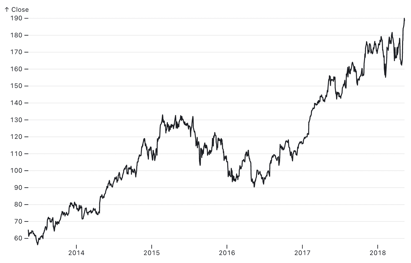
A line chart visualizing the change of Apple’s stock price over time.
Most data visualization libraries connect records in line charts with a straight line from point-to-point by default. For high-frequency time series data collected at predictable intervals, this is often the best choice. However, there may be scenarios where you want to change how the line is drawn between points, such as if you want to visually indicate stepwise changes.
Try it for yourself: To build your own line chart using Observable Plot, simply copy the below example snippet into a JavaScript cell in an Observable Notebook, or select “Line chart” from the cell menu. Connect your data, and update the data and variable names to match what’s in your data. Plot will automatically generate a time series line chart handling scales, axes, and tooltips.
Plot.plot({
  marks: [
    Plot.ruleY([0]),
    Plot.lineY(aapl, { x: "Date", y: "Close", tip: true })
  ]
})
Plot also offers over 20 curve options, which determines how values between points are interpolated. To update your chart using any of the built-in curves, simply add your preferred curve type as an option within your line mark.
Sparklines
For a compact alternative to traditional line charts, consider sparklines. Sparklines are miniature charts that are ideal for showing trends across multiple categories in tight spaces. Since they often omit axes and labels, they're best used when the goal is to highlight general patterns.
Bar charts
While line charts are common, they’re not always the most effective choice. Bar charts are typically used for categorical domains, but they can also visualize aggregated data over time, such as a company’s total month-to-month or quarterly sales by binning the data. Plus, bar charts can be more legible than line charts when there are fewer values to display.
To go deeper into the decision about when to choose a line chart or a bar chart, check out important considerations in this blog.
The best charts for categorical data
Bar charts
As mentioned above, bar charts are most frequently used to visualize categorical data by displaying numeric values grouped by category. For example, you might use a bar chart to show product engagement by user profile, or the number of churned customers by subscription type.
The length of each bar represents a numeric value, which can come from two sources:
An pre-calculated value by group, like a sum, count, or mean, for a numeric column in the data, such as "product visits."
A count of how many records fall into a given category, like the number of tickets labeled "technical issue."
The categorical axis organizes the data into distinct groups that can be ordered in whatever arrangement will be most useful to the viewer. For example, the bars may be sorted by the value that's represented in either ascending or descending order, or they may be sorted by the labels on the categories.
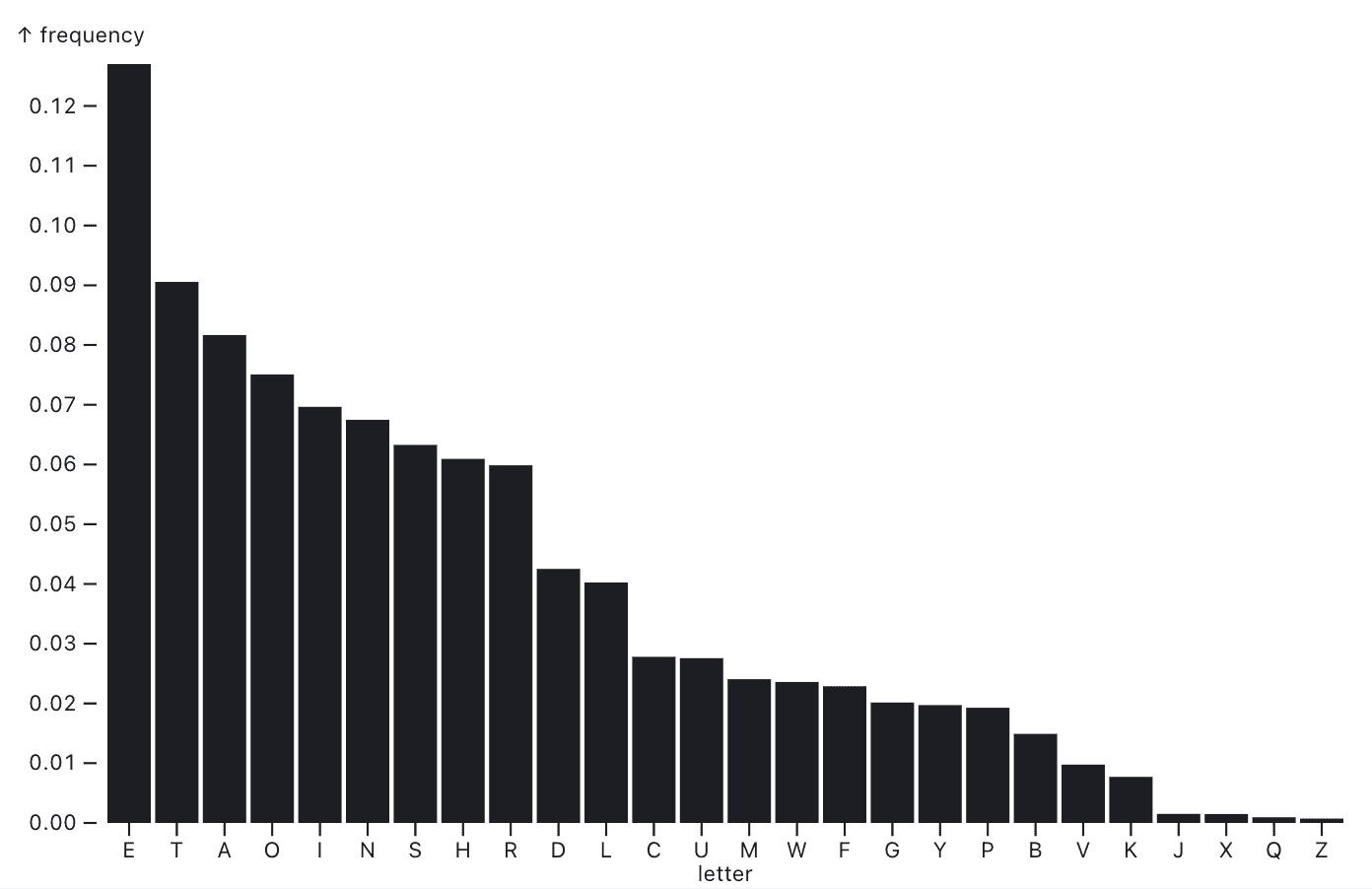
Bar chart showing the distribution of letter frequencies in an English-language corpus.
In some cases, a horizontal bar chart is preferred, for example to avoid overlapping x-axis labels when you have long category names. There are many variations on the bar chart, including the stacked bar chart (which we describe in greater depth below) to show the breakdown of values by subcategories within each group.
See more bar charts examples, including a diverging bar chart and a grouped bar chart, in the Observable Plot gallery.
Radar charts
Radar charts are polar line charts that represent categorical data. While they may look interesting, radar charts should generally be avoided because the order of data dimensions can impact how the data is interpreted. Learn more about why radar charts are usually not the best choice.
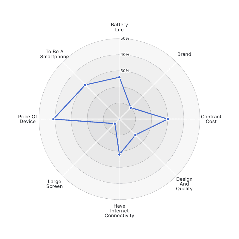
A radar chart showing the results of a survey of smartphone buyers.
The best charts for part-to-whole relationships
When you want to compare how individual components relate to the overall total, you should reach for visualizations that display the size of each part relative to the whole, how each part contributes to the total, and how the whole value is divided across categories.
Stacked bar charts
Stacked bar charts add a fill color or style to each bar that differentiates subcategories within each group. Stacked bars can show absolute values like counts or sums for each subcategory, or stacked values can be normalized to more clearly show proportions. For example, the normalized stacked bar chart below, which uses stack options in Observable Plot to normalize values, shows the proportions of U.S. dams with low, significant, or high risk classification between different dam types:
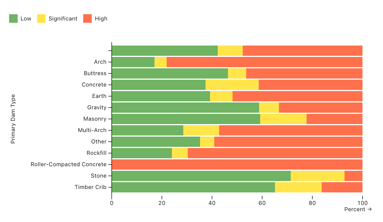
Here's the Observable Plot code we used to create this stacked bar chart:
Plot.plot({
  marginLeft: 180,
  x: { percent: true, label: "Percent" },
  color: {
    legend: true,
    domain: ["Low", "Significant", "High"],
    range: ["#70B362", "#FFE54A", "#FF704D"]
  },
  marks: [
    Plot.barX(
      dams,
      Plot.groupY(
        { x: "count" },
        {
          filter: (d) => d["Hazard Potential Classification"] != "Undetermined",
          y: "Primary Dam Type",
          fill: "Hazard Potential Classification",
          offset: "normalize"
        }
      )
    ),
    Plot.ruleX([0])
  ]
})
Pie charts
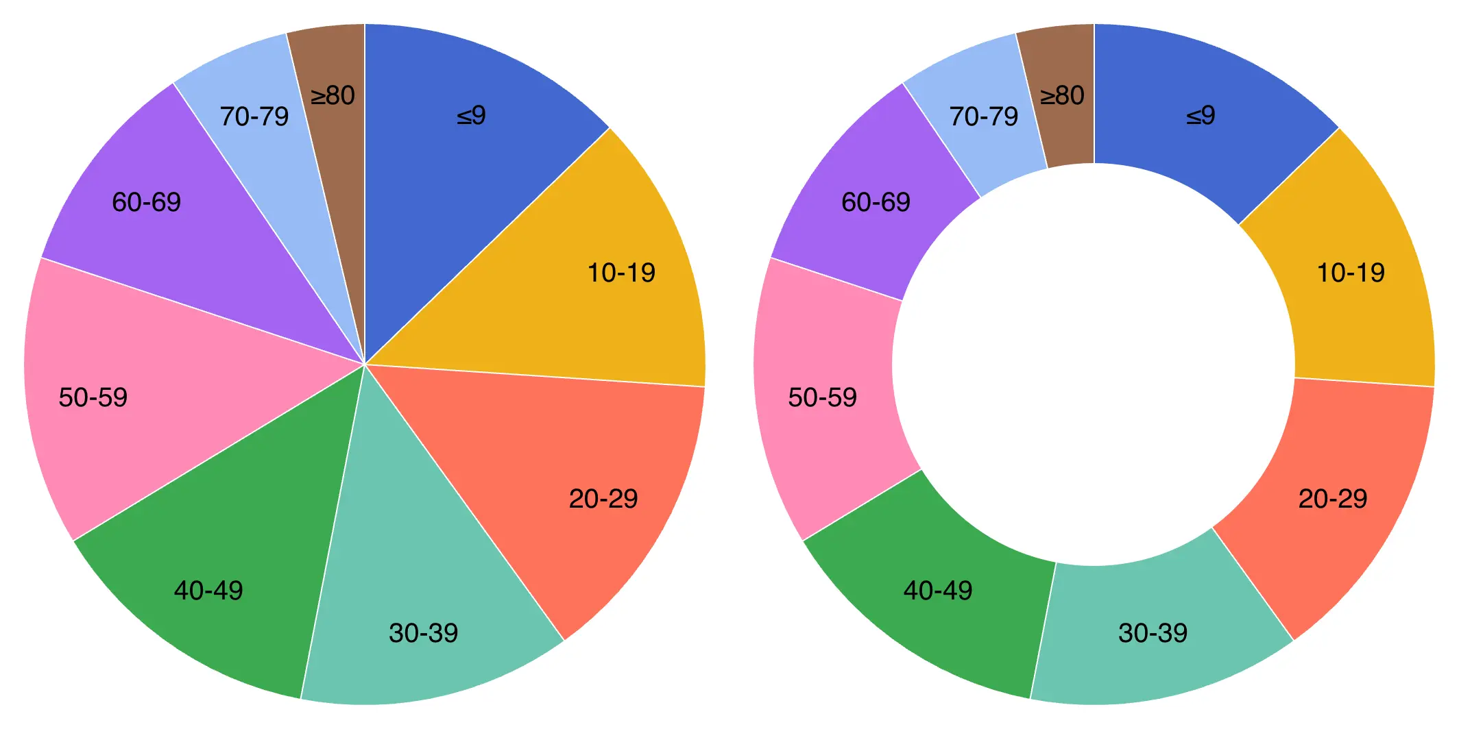
While commonly used, pie charts are often criticized within data visualization circles due to a perception that they can be difficult to accurately interpret.
Pie charts work best with the number of parts (slices in the pie) are fewer, when there are clear differences in proportions by section, and when the different parts add up to 100%. Donut charts are a common variant of the pie chart without the center.
Donut charts are sometimes used for a better data-ink ratio, or when analysts want to add an additional summary value in the center.
Get a primer on why pie charts are controversial in this post.
Waffle charts
Waffle charts represent parts of a whole in a digestible, grid format that allows viewers to more easily infer exact proportions.
In waffle charts, values are broken down into equally sized cells, often squares, that can be quickly counted and compared across groups. For example, the waffle chart below shows the proportions of U.S. dams with low, significant, or high risk potential classifications for the top five most common dam categories with each circle representing ten dams.
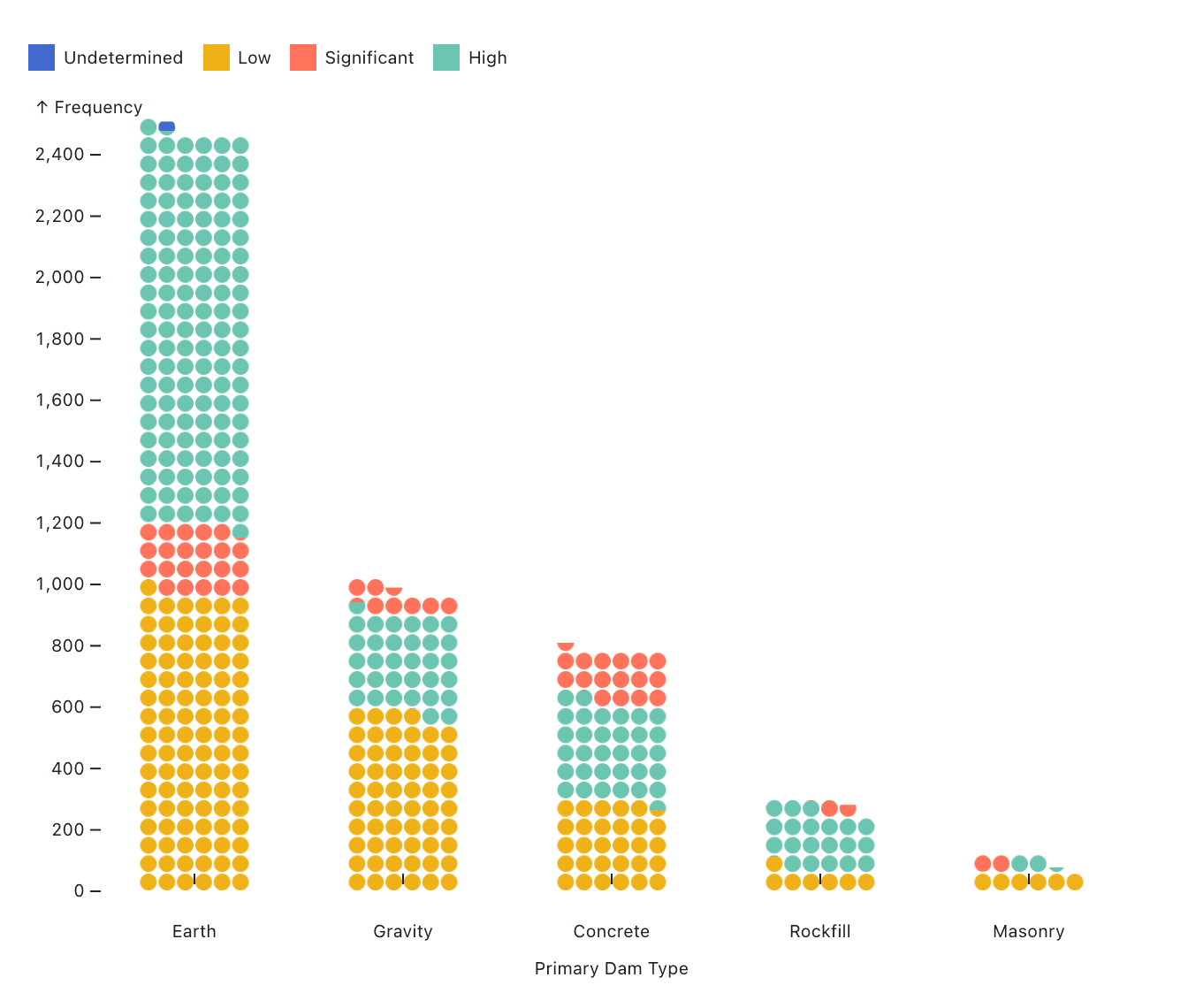
Data: U.S. National Inventory of Dams
You can quickly make waffle charts in Observable Plot using the waffle mark. Customize your chart with built-in options for units (the counts or amount each cell represents), gap size between cells, value rounding to avoid partial shapes, and more.
The best charts for hierarchical data
Hierarchical data represents parent-child relationships.
Treemaps
A treemap subdivides space to show the proportions of a value as part of the whole for hierarchical data. For example, to visualize sales by department and product, the area of each rectangle would show the amount of sales for each, as a fraction of the total sales shown in the chart. Unlike some other chart types, treemaps are also good for packing information in small spaces.
In the example treemap of orders in our Pizza Paradise demo dataset, color represents the pizza category, and each category is further subdivided by pizza type. Rectangle size represents the number of orders for each.
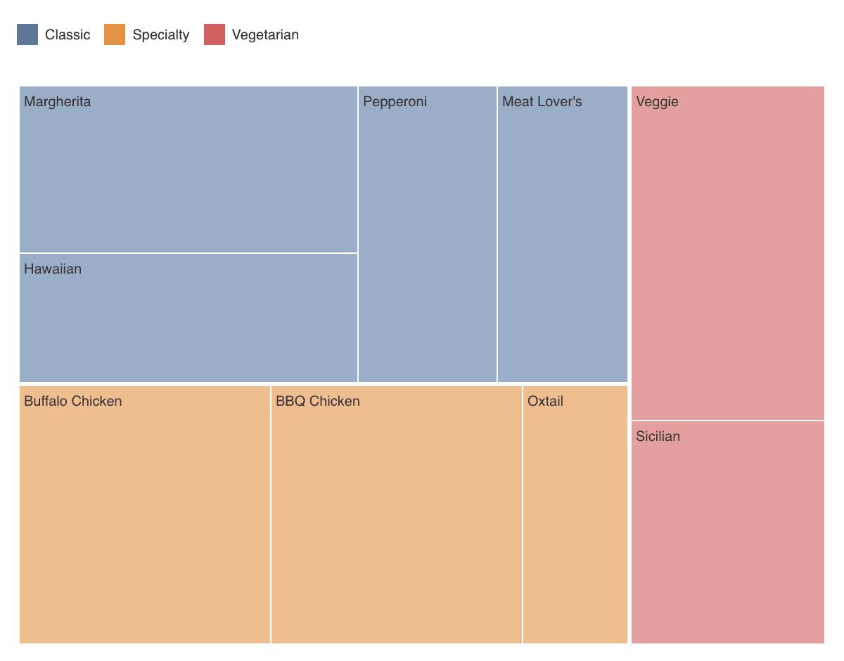
This example treemap is relatively basic; to see more complex variants, such as cascaded and nested treemaps, visit the D3 gallery.
Circle packing charts
A circle packing chart is an alternative to a treemap that visualizes hierarchical data as nested circles, with circle size typically reflecting a quantitative value (such as a count or sum) for each group. While circle packing charts use space less efficiently than treemaps, they can sometimes make it easier for your user to interpret hierarchy. If this chart type is new to you, be sure to check out pro tips for creating circle packing charts in this Observable Notebook.
Sunburst charts
Another type of chart that works well for hierarchical data is the sunburst chart, which consists of a series of concentric rings that correspond to a level in the hierarchy.
Each ring is divided into slices, which can be sized equally or proportionally, depending on an associated value. Sunburst charts can be static, or they can be interactive. For instance, this zoomable sunburst displays just two layers of hierarchy at once, with the ability to zoom in or out for more detail.
A slightly different take on a sunburst is the icicle diagram.
The best charts for geospatial data
There are many ways to visualize geospatial data, but here are five different map types to get you started.
Choropleth maps
A choropleth map uses colors, shades, or patterns to show how a data variable changes across different geographic regions. They help reveal patterns or differences in the data by using color progressions — such as light to dark or one hue to another — to represent varying values.
One consideration to keep in mind when building choropleths is that they can make it difficult to read exact values and larger areas can appear more important than smaller ones (even if the data doesn’t support that). To get started creating your own choropleth, check out this Observable Plot tutorial.
Bubble maps
To show magnitude and compare proportions across geographic regions, you may want to choose a bubble map.
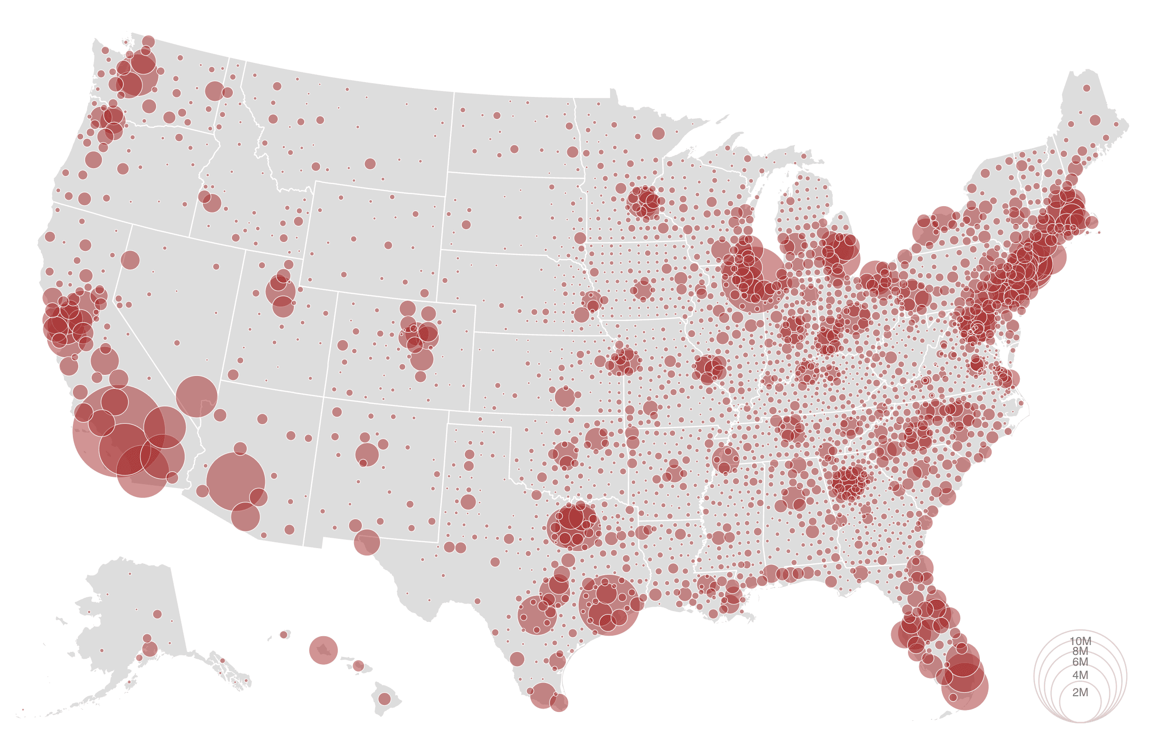
Estimated population by county, 2016
Similar to a bubble map, a spike map uses vertical spikes to represent quantitative values, with the spike height corresponding to a specific data value. Instead of using area to encode data, like bubble maps, the spike height can reduce overlap in dense areas, making them a good choice for datasets like population density.
Arc maps
An arc map visualizes flows or connections between locations. In the example below, the map shows seafood imports to the United States, with arc thickness and color dependent on import volume from each exporting country (in kilograms).
Grid cartograms
A grid cartogram represents subregions using tiles of the same shape, arranged to reflect their general geographic locations while avoiding overlap. The most common tile shapes are squares and hexagons, but they can also be rectangle cartograms, dot cartograms, and more.
The biggest drawback to grid cartograms is that they aren’t geographically accurate representations. But, they have numerous benefits — such as helping viewers compare values between regions and creating equal representation between smaller and larger regions.
If these examples have sparked a deeper curiosity about map-making, then you won’t want to miss this interview with data visualization developer Fil Rivière and this video about using dynamic cartograms to visualize election data.
The best charts for distribution of values
Histograms
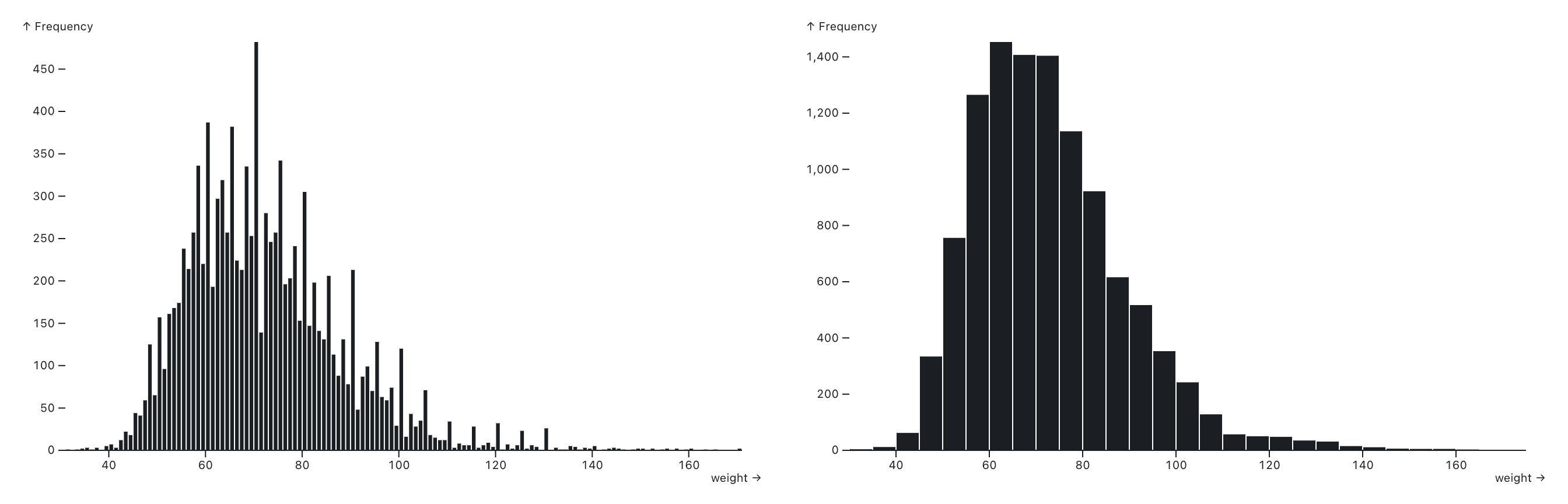
One of the most useful data visualization types for demonstrating how values are distributed, and the shape of that distribution is the histogram. In histograms, data is grouped into bins that display the count of how many data points are in each bin.
Beeswarms
A visually interesting alternative to other charts that show a distribution of values is the beeswarm, which visualizes observations for a single quantitative variable and uses jitter to avoid overlapping marks. Encodings for color and size can represent additional variables in the chart.
The beeswarm chart below visualizes the distribution of product price by category.
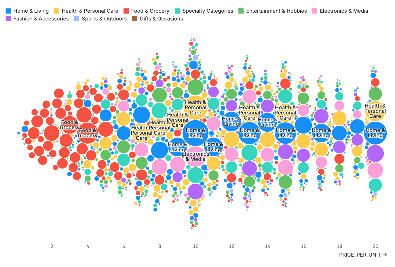
Data: Amazon e-commerce data
Data: Amazon e-commerce data
Box plots
Another alternative to a histogram for visualizing distribution of values is the box plot, sometimes called a box-and-whisker plot, which summarizes quantitative distribution using boxes and lines (“whiskers”) to visualize the spread of the data. In this example from the D3 gallery, the price distribution (y-axis) of a set of diamonds is plotted for a given range of carat values (x-axis).
The best charts for showing relationships between variables
Scatter plots
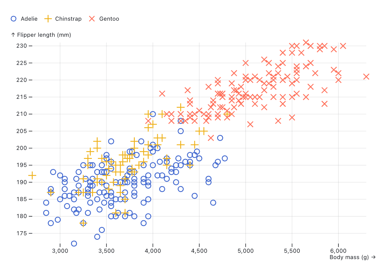
To visualize correlations or patterns between two numeric variables, data analysts will oftentimes choose a scatter plot.
In scatter plots, data is shown on two continuous axes with each data point plotted so that its horizontal and vertical positions represent the values of the two chosen data dimensions. Color or symbols can also be used to encode specific variables as is done, for instance, in this example that visualizes flipper length and body mass for different types of penguins.
The best charts for showing changes in rankings
Bump charts
Bump charts show changes in rankings by group, usually over time. For example, a bump chart might visualize shifts in product rankings by annual volume sold, or changes in how survey participants rate the importance of issues (like economy, environment, education, healthcare, or foreign policy) when considering political candidates.
In the bump chart below, we can track the rankings for selected U.S. seafood imports over time by product:
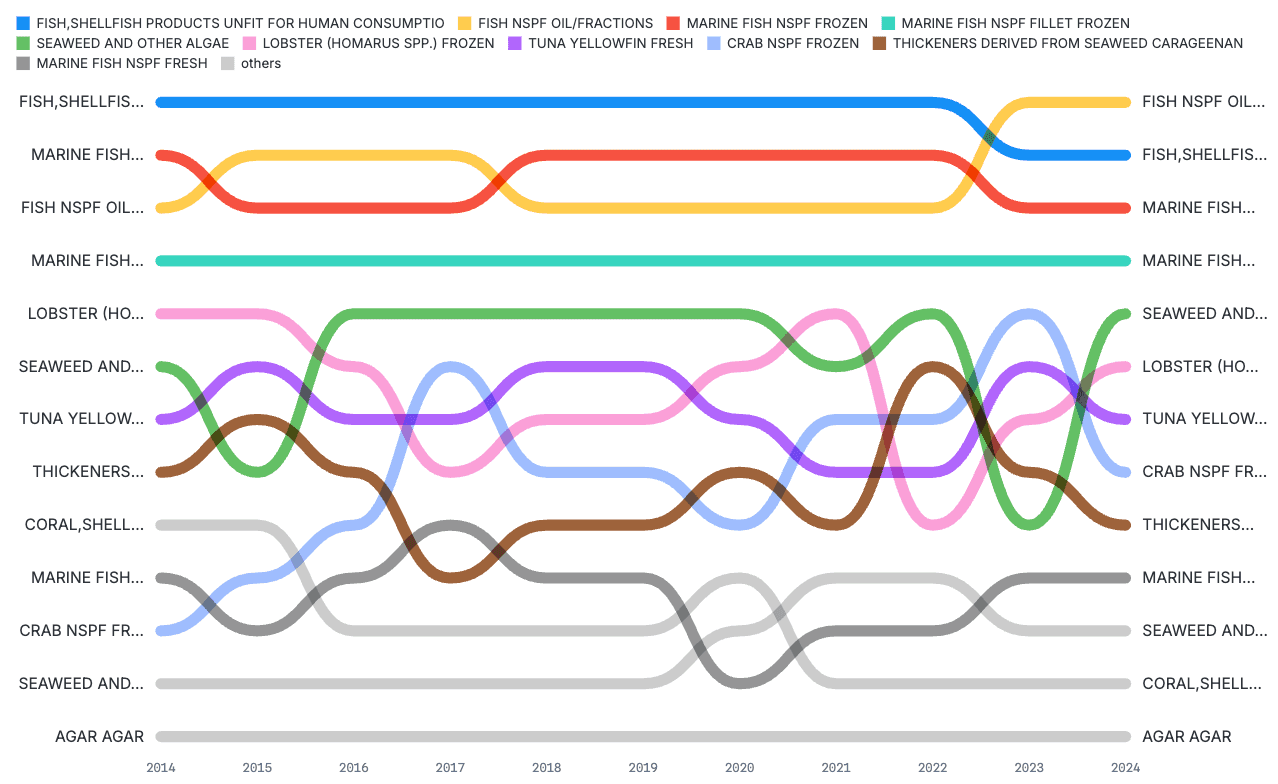
Data: NOAA US Trade in Fishery Products
Conclusion
Selecting the right chart type for your data is a fundamental part of data exploration, analysis, and communication. Once you’ve selected the best chart for your dataset, you can start evaluating whether or not to add additional elements, like brushing, animations, or interactivity.
To start building the more advanced chart types covered in this post, explore and fork notebooks from our D3 and Plot galleries: